An optimization algorithm for deriving the average flow velocity in a shallow microchannel through spatiotemporal concentration gradient
-
摘要: 微流控通道内流速的准确测量在利用微流控芯片开展定量化学分析、样品制备、药物合成等领域具有重要应用价值。基于物质输运原理,提出了一种通过测量物质时空浓度梯度反演扁平微通道中平均流速的优化算法。首先,基于Navier-Stokes方程与Taylor-Aris弥散方程建立扁平微通道中速度场与浓度场的定量关系,分别提出了用直接反演法和优化算法求解平均流速的方法;其次,通过数值仿真系统地分析了时空浓度变化频率、振幅和扩散系数对反演流速准确度的影响;最后,通过荧光素实验验证了该方法的可行性。结果表明:无噪声情况下,优化算法反演结果与真实速度相关系数为1,具有很高的精度;有噪声情况下,增大物质浓度信号的频率与振幅、采用扩散系数较小的物质有助于提高算法的准确度;在微流控装置中,优化算法反演结果与流量传感器测量计算结果的相关系数为0.9814。
-
关键词:
- 流速测量 /
- 扁平微通道 /
- Taylor-Aris弥散 /
- 优化算法 /
- 时空浓度梯度
Abstract: Precise measurement of the flow velocity in microfluidic channels plays an important role in the application of microfluidic chips for quantitative chemical analysis, sample preparation, drug synthesis, etc. In this study, based on the principle of mass transport in microchannels, an optimization algorithm is proposed to derive the average flow velocity within a shallow microchannel through the spatiotemporal concentration gradient. Firstly, based on the relationship between the flow field and the concentration field in the shallow microchannel governed by the Navier-Stokes equation and the Taylor-Aris dispersion equation, a direct inversion method and an optimization algorithm to derive the average flow velocity are demonstrated respectively. Secondly, the influence of the parameters of the spatiotemporal concentration signals (i.e. frequency, amplitude and diffusion coefficient) on the prediction accuracy of the average velocity has been analyzed using numerical simulation. Finally, experiments using fluorescent dye are carried out to verify the feasibility of the proposed method. Simulation results show that the correlation coefficient between the derived average velocity obtained by the optimization algorithm and the real velocity is one in the absence of noise interference, which indicates high calculation accuracy. In the case of noise interference, the accuracy of the optimization algorithm can be improved by increasing the frequency and amplitude of the dynamic concentration. And a low diffusion coefficient can also improve the accuracy. In the microfluidic experiments, a correlation coefficient between the inversion result of the optimization algorithm and the measurement of the flow sensor can be as high as 0.9814. -
0 引 言
近年来,随着微流控芯片技术在化学、生命科学、医学等相关领域的广泛应用,微流控通道内流体的定量检测与精确操控已成为重要的研究热点[1]。速度是流场最主要的特征参数之一,因此微流控通道内流速的测量对于研究微量多相流体的精准操控、构建复杂的离体生物力学微环境、控制生化反应过程等都具有重要意义[2-4]。高度远小于横向和纵向几何尺寸的扁平微通道是最常见的微通道结构形式,其高度方向的平均流速测量是定量分析壁面剪切力和物质输运规律的前提[5-7]。
常见的流速测量方法是通过测量粒子跟随流体的运动来实现,例如微尺度粒子图像测速法(micro-PIV)和微尺度粒子跟踪测速法(micro-PTV)。前者通过连续拍摄记录流场中的粒子群,比较相邻时间间隔的粒子群位置变化来计算流体速度[8];后者采用拉格朗日类方法直接测量分析单个粒子的运动,避免了micro-PIV的平均效应,实现了更高的空间精度[9-10]。但这类基于粒子的测速方法在测量小尺度结构时存在较大误差,因为测量小尺度的流动特性需要较大的示踪粒子浓度,但过大的粒子浓度会引发激光穿透困难等问题。此外,这类方法的测量精度还受示踪粒子跟随性的影响[11-13]。随着光学技术的快速发展,科研人员提出了点检测扫描方法[14]。该方法利用光学仪器对准激光进行强聚焦,可以实现高分辨率的单点速度测量,但对系统的校准精度要求较高,且设备昂贵、操作复杂。常见的测量方法还有标量图像测速法,其原理是从守恒标量(如浓度、厚度)的观测中获取速度[15]。与基于粒子的测速技术相比,该方法不存在由粒子尺寸带来的流场干扰和跟随性误差,可以更精确地实现流速测量,已被广泛应用于湍流研究和天气预报[16-17];而在微流控通道内主要是低雷诺数的层流,标量图像的时空分布必然受流体对流-扩散的共同作用,特别是在扩散占优的流动条件下,标量场的时空梯度分布与流场之间的耦合关系变得相对复杂,如何依据标量场的时空分布确定微通道内的流体流动信息及相关影响因素尚有待于进一步研究。
为实现扁平微通道内流速的精确测量,本文以标量图像测速法为基础,结合微通道内物质输运原理,提出了一种基于时空浓度梯度反演扁平微通道中平均流速的优化算法。通过光学成像技术获得微通道内物质的时空浓度梯度,利用扁平微通道结构特点,基于Taylor-Aris弥散方程得到描述物质浓度与平均流速间的定量关系,结合优化问题中最小化目标函数的思想,计算得出扁平微通道内流体的平均流速。通过数值仿真验证该优化算法在无噪声条件下的可行性和精度,分析噪声条件下输入浓度信号和物质扩散系数对算法求解准确度的影响。最后利用提出的方法分析微通道中物质浓度图像的时间序列,将优化算法反演得到的流速与流量传感器测量计算结果进行比较,验证算法的可行性和准确性。
1 基于浓度场反演流速的方法
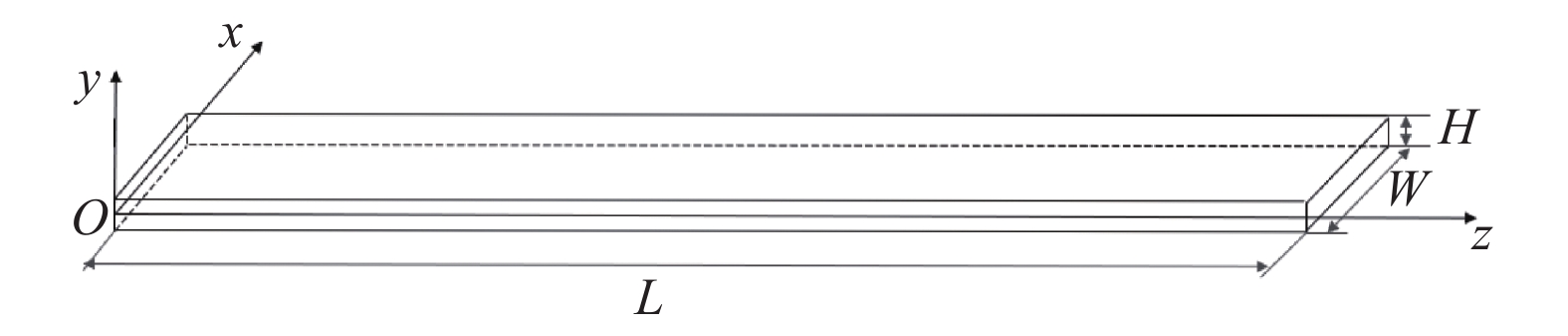
为了获得微通道内浓度场与平均流速之间的定量关系,首先基于Navier-Stokes方程和Taylor-Aris弥散方程构建流道模型并进行理论分析。待检测的扁平直通道如图1所示,其高为H,宽为W,长为L。
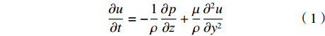
扁平微通道满足H<<W、H<<L,忽略通道侧面边界的影响,流体运动仅受上下流道壁面的黏性力及z方向驱动压力差的影响。此时,微通道内流体流动的控制方程可简化为[18]:
$$ \frac{{\partial u}}{{\partial t}} = - \frac{1}{\rho }\frac{{\partial p}}{{\partial {\textit{z}}}} + \frac{\mu }{\rho }\frac{{{\partial ^2}u}}{{\partial {y^2}}} $$ (1) 其中,
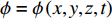
$ u = u\left( {y,t} \right) $ 为z方向的流速,$p = p\left( {{\textit{z}},t} \right)$ 为压力,$\; \rho $ 为流体密度,$\; \mu $ 为流体动力黏度,$t $ 为时间。在扁平微通道的入口边界处加载浓度随时间变化的物质溶液,物质在微通道中受到对流和扩散的影响,物质浓度
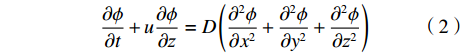
$\phi = \phi \left( {x,y,{\textit{z}},t} \right)$ 满足对流-扩散方程[19]:$$ \frac{{\partial \phi }}{{\partial t}} + u\frac{{\partial \phi }}{{\partial {\textit{z}}}} = D\left( {\frac{{{\partial ^2}\phi }}{{\partial {x^2}}} + \frac{{{\partial ^2}\phi }}{{\partial {y^2}}} + \frac{{{\partial ^2}\phi }}{{\partial {{\textit{z}}^2}}}} \right) $$ (2) 其中,
$D $ 为物质的扩散系数。微通道的高度H很小,物质在y方向可视为均匀分布,以平均浓度
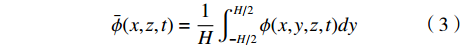
$\bar \phi = \bar \phi \left( {x,{\textit{z}},t} \right)$ 表示:$$ \bar \phi (x,{\textit{z}},t) = \frac{1}{H}\int_{ - H/2}^{H/2} \phi (x,y,{\textit{z}},t)dy $$ (3) 微通道几何尺寸在微米量级且z方向的流速较小,Re << 1,满足小雷诺数流动条件;进一步假定微通道中的流动满足准定常条件[20],因此微通道中的流速
$u $ 满足:$$ u = \frac{{3\bar u}}{2}\left[ {1 - {{\left( {\frac{{2y}}{H}} \right)}^2}} \right] $$ (4) 其中,
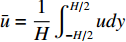
$\bar u = \dfrac{1}{H}\displaystyle\int_{ - H/2}^{H/2} u dy$ 为y方向的平均流速。结合式(2)~(4)化简可得Taylor-Aris弥散方程:
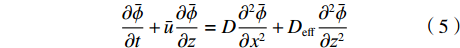
$$ \frac{{\partial \bar \phi }}{{\partial t}} + \bar u\frac{{\partial \bar \phi }}{{\partial {\textit{z}}}} = D\frac{{{\partial ^2}\bar \phi }}{{\partial {x^2}}} + {D_{{\rm{eff}}}}\frac{{{\partial ^2}\bar \phi }}{{\partial {{\textit{z}}^2}}} $$ (5) 其中
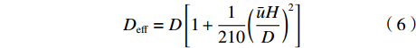
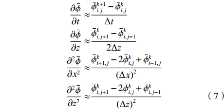
$D_{{\rm{eff}}}$ 称为有效扩散系数,满足:$$ {D_{{\rm{eff}}}} = D\left[ {1 + \frac{1}{{210}}{{\left( {\frac{{\bar uH}}{D}} \right)}^2}} \right] $$ (6) 将式(5)进行差分展开,以横向的空间步长Δx将流道区域沿x方向均匀离散成Nx份,网格点为xi ,其中i=1,2,···,(Nx+1);以纵向的空间步长Δz将流道区域沿z方向均匀离散成Nz份,网格点为zj ,其中j=1,2,···,(Nz+1);同时用时间步长Δt将时间t均匀离散为Nt份,时间网格点为tk ,其中k=1,2,···,(Nt+1)。根据有限差分原理,浓度的一阶和二阶导数可近似展开为:
$$ \begin{split} \dfrac{{\partial \bar \phi }}{{\partial t}} \approx& \dfrac{{\bar \phi _{i,j}^{k + 1} - \bar \phi _{i,j}^k}}{{\Delta t}}\\ \dfrac{{\partial \bar \phi }}{{\partial {\textit{z}}}} \approx& \dfrac{{\bar \phi _{i,j + 1}^k - \bar \phi _{i,j - 1}^k}}{{2\Delta {\textit{z}}}}\\ \dfrac{{{\partial ^2}\bar \phi }}{{\partial {x^2}}} \approx& \dfrac{{\bar \phi _{i + 1,j}^k - 2\bar \phi _{i,j}^k + \bar \phi _{i - 1,j}^k}}{{{{(\Delta x)}^2}}}\\ \dfrac{{{\partial ^2}\bar \phi }}{{\partial {{\textit{z}}^2}}} \approx& \dfrac{{\bar \phi _{i,j + 1}^k - 2\bar \phi _{i.j}^k + \bar \phi _{i,j - 1}^k}}{{{{(\Delta {\textit{z}})}^2}}} \end{split} $$ (7) 式(5)可整理为:
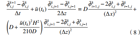
$$ \begin{split}& \frac{{\bar \phi _{i,j}^{k + 1} - \bar \phi _{i,j}^k}}{{\Delta t}} + \bar u\left( {{t_k}} \right)\frac{{\bar \phi _{i,j + 1}^k - \bar \phi _{i,j - 1}^k}}{{2\Delta {\textit{z}}}} = D\frac{{\bar \phi _{i + 1,j}^k - 2\bar \phi _{i,j}^k + \bar \phi _{i - 1,j}^k}}{{{{(\Delta x)}^2}}} + \\& \left( {D + \frac{{\bar u{{\left( {{t_k}} \right)}^2}{H^2}}}{{210D}}} \right)\frac{{\bar \phi _{i,j + 1}^k - 2\bar \phi _{i,j}^k + \bar \phi _{i,j - 1}^k}}{{{{(\Delta {\textit{z}})}^2}}}\\[-10pt] \end{split} $$ (8) 其中,
${\bar \phi _{i + 1,j}^k} $ 、${\bar \phi _{i,j}^k} $ 、$ {\bar \phi _{i - 1,j}^k}$ 分别表示tk时刻、长度方向zj处、宽度方向xi+1、xi、xi–1处的物质浓度;${\bar \phi _{i,j + 1}^k} $ 、${\bar \phi _{i,j - 1}^k} $ 分别表示tk时刻、宽度方向xi处、长度方向zj+1、zj–1处的物质浓度;${\bar \phi _{i,j}^{k + 1}} $ 表示tk+1时刻xi 、zj处的物质浓度。通过光学成像技术得到流道中固定时间间隔$ \Delta t$ 对应的物质浓度图像的时间序列,把图像中每个像素点的物质浓度作为${\bar \phi _{i,j}^k} $ ,相邻像素间的距离作为$\Delta x $ 和$\Delta {\textit{z}}$ ,采样间隔作为$\Delta t $ ,利用式(8)即可计算微通道中的平均速度$\bar u $ 。1.1 直接反演法
将式(8)整理为关于平均流速
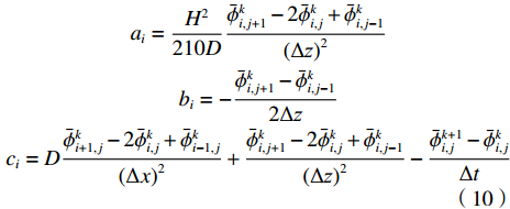
$\bar u $ 的一元二次方程形式:$$ {a_i}\bar u{\left( {{t_k}} \right)^2} + {b_i}\bar u\left( {{t_k}} \right) + {c_i} = 0 $$ (9) 式中,各系数表达式如下:
$$ \begin{gathered} {a_i} = \frac{{{H^2}}}{{210D}}\frac{{\bar \phi _{i,j + 1}^k - 2\bar \phi _{i,j}^k + \bar \phi _{i,j - 1}^k}}{{{{(\Delta {\textit{z}})}^2}}}\\ {b_i} = - \frac{{\bar \phi _{i,j + 1}^k - \bar \phi _{i,j - 1}^k}}{{2\Delta {\textit{z}}}}\\ {c_i} = D\frac{{\bar \phi _{i + 1,j}^k - 2\bar \phi _{i,j}^k + \bar \phi _{i - 1,j}^k}}{{{{(\Delta x)}^2}}} + \frac{{\bar \phi _{i,j + 1}^k - 2\bar \phi _{i,j}^k + \bar \phi _{i,j - 1}^k}}{{{{(\Delta {\textit{z}})}^2}}} - \frac{{\bar \phi _{i,j}^{k + 1} - \bar \phi _{i,j}^k}}{{\Delta t}} \end{gathered} $$ (10) 直接反演法利用各时刻微通道内浓度
$ {\bar \phi _{i,j}^k}$ ,通过求解一元二次方程得到每一时刻的平均流速${\bar u} $ 。1.2 优化算法
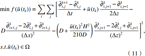
结合优化问题的思想,提出一种新的求解方法,构造如下的平均流速优化问题:
$$\begin{split}& {\rm{min}}\;f\left( {\bar u\left( {{t_k}} \right)} \right) = \sum\limits_i {\sum\limits_j {} } \left[ {\frac{{\bar \phi _{i,j}^{k + 1} - \bar \phi _{i,j}^k}}{{\Delta t}} + \bar u\left( {{t_k}} \right)\frac{{\bar \phi _{i,j + 1}^k - \bar \phi _{i,j - 1}^k}}{{2\Delta {\textit{z}}}} - } \right.\\& {\left. D\frac{{\bar \phi _{i + 1,j}^k - 2\bar \phi _{i,j}^k + \bar \phi _{i - 1,j}^k}}{{{{(\Delta x)}^2}}} -{\left( {D + \frac{{\bar u{{\left( {{t_k}} \right)}^2}{H^2}}}{{210D}}} \right)\frac{{\bar \phi _{i,j + 1}^k - 2\bar \phi _{i.j}^k + \bar \phi _{i,j - 1}^k}}{{{{(\Delta {\textit{z}})}^2}}}} \right]^2}, \\& {s.t.\bar u\left( {{t_k}} \right) \in \Omega } \end{split} $$ (11) 其中,
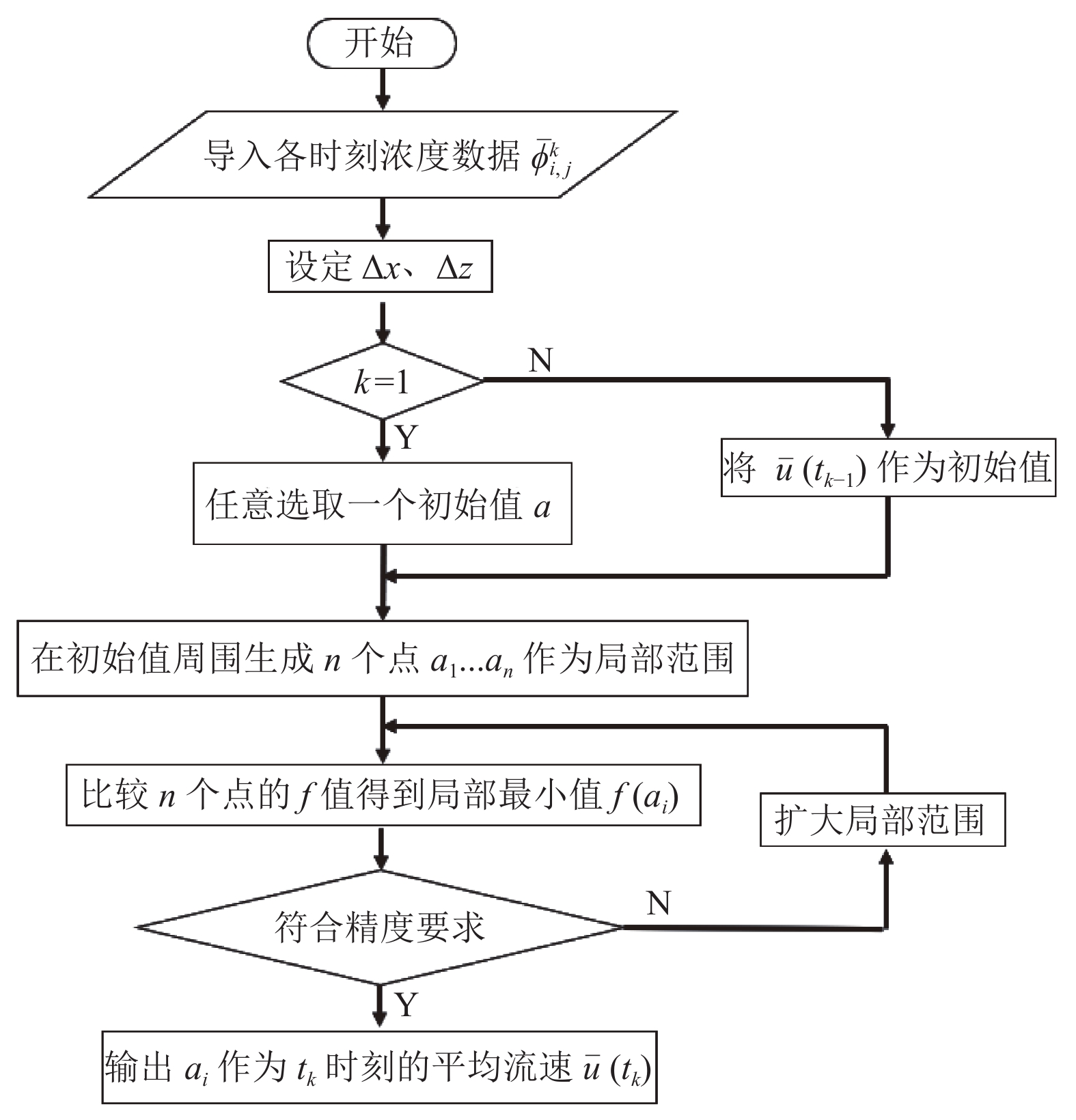
$f\left( {\bar u\left( {{t_k}} \right)} \right) $ 为目标函数,$\Omega $ 为约束条件:$\dfrac{{\partial u}}{{\partial {\textit{z}}}} = $ $ \dfrac{{\partial u}}{{\partial x}} = 0$ 。代入浓度时空分布数据,设置优化参数,使用优化算法在约束条件下对目标函数进行优化求解,得到tk时刻平均流速
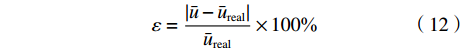
$ \bar u\left( {{t_k}} \right)$ ,优化算法流程如图2所示。对于定常流动情况,定义相对误差
$\varepsilon $ 来表征优化算法的精度:$$ \varepsilon = \frac{{\left| {\bar u - {{\bar u}_{{{{\rm{real}} }}}}} \right|}}{{{{\bar u}_{{{{\rm{real}} }}}}}} \times 100{\text{%}} $$ (12) 对于脉动流情况,定义相关系数R来表征优化算法的精度:
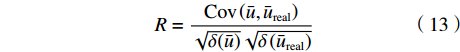
$$ R = \frac{{{\rm{Cov}}\left( {\bar u,{{\bar u}_{{\rm{real}}}}} \right)}}{{\sqrt {\delta (\bar u)} \sqrt {\delta \left( {{{\bar u}_{{\rm{real}}{\rm{ }}}}} \right)} }} $$ (13) 其中,
$\bar u $ 表示通过优化算法求解的平均流速,${{{\bar u}_{{\rm{real}}{\rm{ }}}}}$ 表示真实的平均流速,Cov表示协方差,δ 表示方差。2 数值仿真
2.1 微通道内时空浓度分布
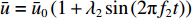
为了研究基于浓度分布反演流速的方法,首先构建了微通道内物质时空浓度分布。以扁平微通道为例构建如图1所示微通道,其长度L为3 cm,宽度W为3 mm,高度H为150 μm。在微通道内给定均匀分布的流速条件,按其形式可分为定常流和脉动流。在脉动流情况下,流速以正弦波形式变化,满足
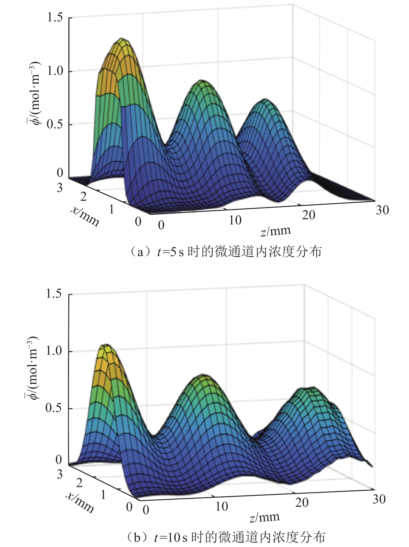
$\bar{u}=\bar{u}_{0} \left(1+\lambda_{2} \sin \left(2 {\text{π}} f_{2} t\right)\right)$ ,其中$\bar{u}_{0} $ 为速度信号的平均值,$\lambda_{2} $ 为速度信号的振幅,$ f_{2} $ 为速度信号的频率。将通道始端正中间宽度为1 mm的区域作为入口,向其通入浓度动态变化的组分,其浓度$\bar{\phi} $ 以正弦波形式变化,满足$\bar{\phi}=\bar{\phi}_{0} \left(1+\lambda_{1} \sin \left(2 {\text{π}} f_{1} t\right)\right)$ ,其中$\bar{\phi}_{0} $ 为浓度信号的平均值,$\lambda_{1} $ 为浓度信号的振幅,$f_{1} $ 为浓度信号的频率。通过MATLAB程序求解式(8),将速度作为已知量迭代求解浓度分布,边界条件设为左右壁面和微通道出口处无浓度梯度,即可得到微通道内时空浓度分布情况。图3为脉动流$\bar u=0.0037(1 + $ $ 0.5\sin (0.1{\text{π}} t))\;{\rm{m}}/{\rm{s}}$ 、入口浓度$\bar{\phi}=1+0.5 \sin (0.1 {\text{π}} t) \ \mathrm{mol} / \mathrm{m}^{3}$ 条件下物质在微通道内传输5 s和10 s后的浓度分布。![]() 图 3 微通道内浓度分布仿真结果Fig. 3 Simulation results of the concentration distribution in the micro-channel
图 3 微通道内浓度分布仿真结果Fig. 3 Simulation results of the concentration distribution in the micro-channel2.2 无噪声条件下流速反演
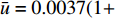
基于构建的微通道内时空浓度分布,分别在定常流和脉动流条件下,对无噪声存在时以直接反演法与优化算法计算平均流速的方法进行了验证。基于动态浓度信号
$\bar{\phi}=1+0.5 \sin (0.1 {\text{π}} t) \ \mathrm{mol} / \mathrm{m}^{3}$ 在定常流中的浓度分布,图4(a)给出了直接反演法和优化算法计算得到的平均流速与真实流速的比较结果。结果表明:直接反演法所求流速在浓度信号处于极值点时有明显误差。原因是当浓度处于极值点时,浓度对时间的导数为零,式(10)中$c_i $ 存在较大误差;此外,一元二次方程的求解存在除法运算,分母$a_i $ 的微小波动也会对结果产生较大影响。相比之下,由优化算法求得的流速与真实流速几乎完全重合,相对误差$\varepsilon $ =0.001%。在脉动流情况下(图4(b)),直接反演法所得流速在特定点处仍存在较大的计算误差,而由优化算法求得的平均流速与真实流速的相关系数R=1,相比于直接反演法有更高的反演精度。![]() 图 4 直接反演法和优化算法求得平均流速与真实流速对比Fig. 4 Comparison between the real velocity and the average velocity derived based on the direct inversion method and the optimiza-tion algorithm
图 4 直接反演法和优化算法求得平均流速与真实流速对比Fig. 4 Comparison between the real velocity and the average velocity derived based on the direct inversion method and the optimiza-tion algorithm2.3 有噪声条件下流速反演
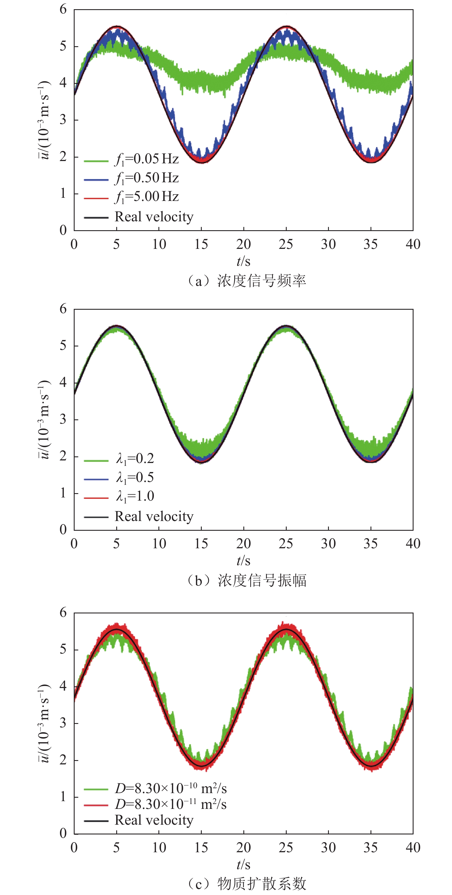
由于实验中测得的时空浓度分布通常存在噪声,因此本节讨论噪声条件下物质浓度信号的频率、振幅和物质扩散系数对流速求解的影响。通过在浓度数据中添加0.1%的白噪声来模拟实验测得浓度数据中的噪声。
入口浓度变化满足
$\bar{\phi}=\bar{\phi}_{0} \left(1+\lambda_{1} \sin \left(2 {\text{π}} f_{1} t\right)\right)$ ,采用控制变量法探究$ f_{1} $ 、$\lambda_{1} $ 和D对优化算法结果准确性的影响,如图5所示。以浓度信号频率为例进行具体分析:当采用的频率较低(即近似于浓度恒定)时,通过优化算法推断的流速与真实流速差距较大,原因在于小雷诺数流动条件下对流不占优,当物质浓度频率较低时,难以形成明显的空间浓度梯度;而当增大频率至5.00 Hz时,推断结果与真实流速基本吻合,这说明该算法对数据的时空分辨率要求较高。![]() 图 5 浓度信号参数对优化算法反演平均流速的影响Fig. 5 Influence of parameters of the concentration signals on the average velocity derived by the optimization algorithm
图 5 浓度信号参数对优化算法反演平均流速的影响Fig. 5 Influence of parameters of the concentration signals on the average velocity derived by the optimization algorithm由仿真结果可知:在噪声条件下,增大物质浓度信号的频率和振幅、选择扩散系数较小的物质可以提升优化算法的准确度。
3 实验验证
3.1 实验装置与方法
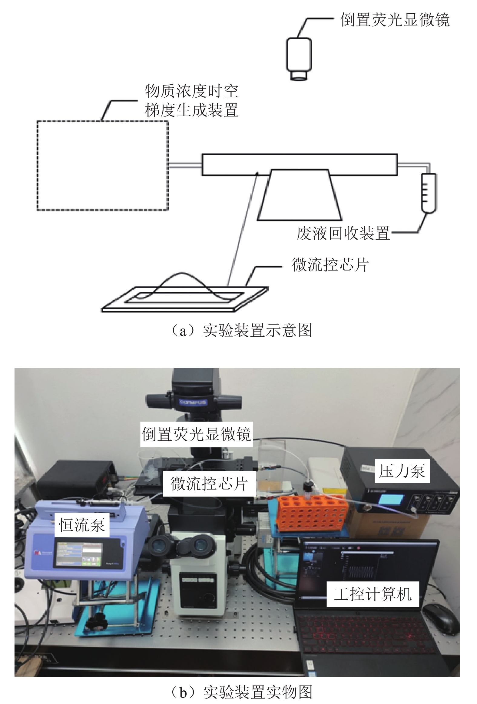
实验装置如图6所示,主要包括物质浓度时空梯度生成装置、具有扁平微通道的微流控芯片、倒置荧光显微镜和废液回收装置。实验中组合使用恒流泵和工控计算机控制的压力泵作为浓度梯度生成装置。
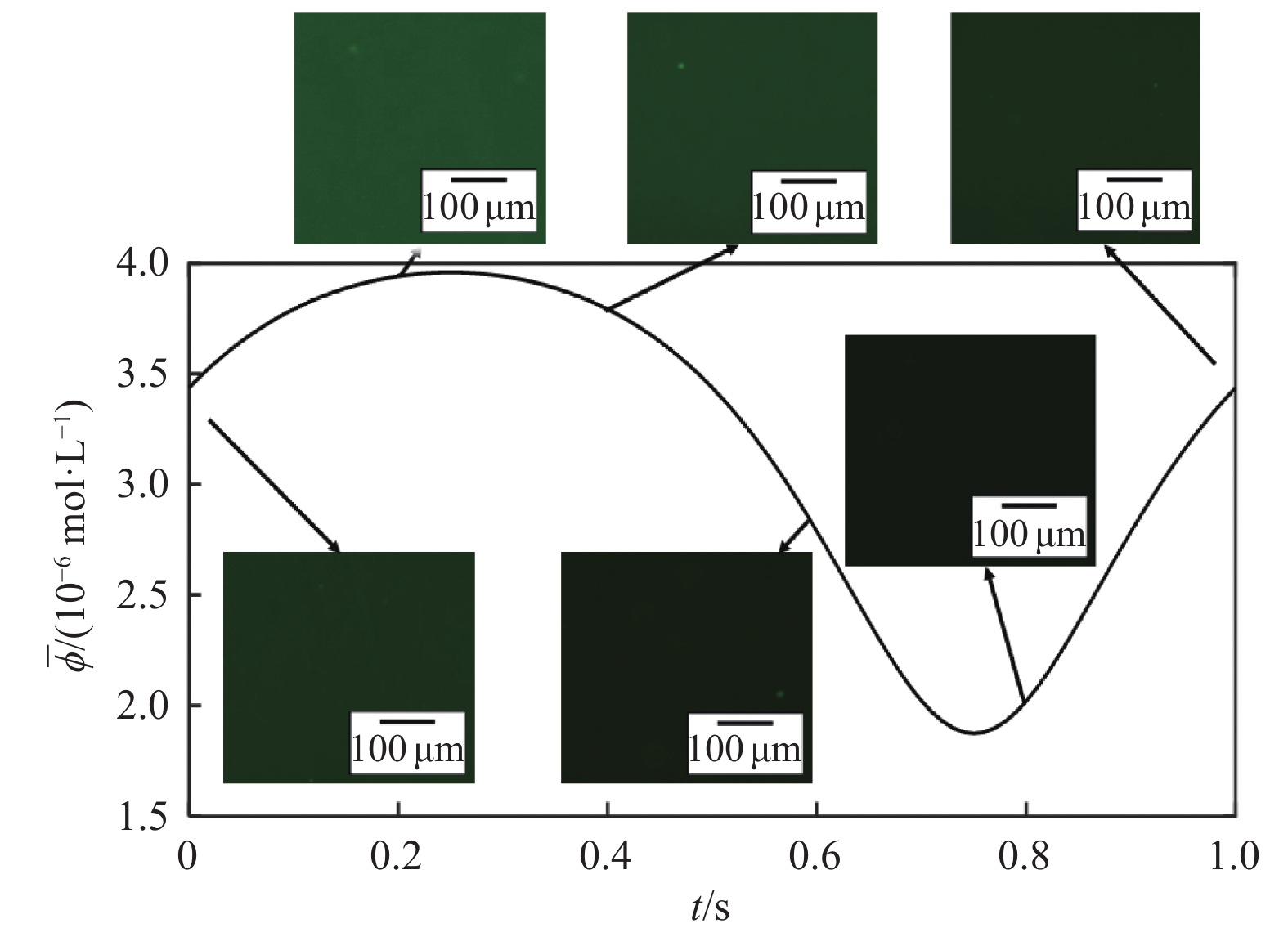
利用该装置确定扁平微通道内平均流速包括以下步骤:在压力泵配套的储液管内加入摩尔浓度为5 ×10⁻⁶ mol/L的罗丹明溶液,其扩散系数为4.14×10–10 m2/s,在恒流泵的注射器中加入去离子水,通过调节参数控制两泵,使其体积流率随时间按照一定规律变化,进而在微通道的入口处产生摩尔浓度随时间变化的罗丹明溶液,由于横向分子扩散效应,最终在扁平微通道中产生时空浓度梯度。待废液回收装置出现液体后,利用倒置荧光显微镜记录距离微通道入口一定长度处的测量视野内不同时刻的罗丹明溶液摩尔浓度分布,进而得到时间间隔为Δt的一系列荧光图像,如图7所示。最后对所得图像进行处理:取不同时刻相同区域的荧光图像,提取灰度值并转化为对应摩尔浓度值后代入优化算法式子中,设置优化参数进行计算,即可得到不同时刻下微通道内的平均流速。
3.2 实验结果
实验时采用的直线型微通道几何尺寸如下:长度4 cm,宽度4 mm,高度80 μm。将距离微通道入口2 cm处作为显微镜观测位置,照片拍摄帧率为13.407 Hz,空间分辨率为4 μm/pixel。实验时拍摄的荧光图像如图8所示。
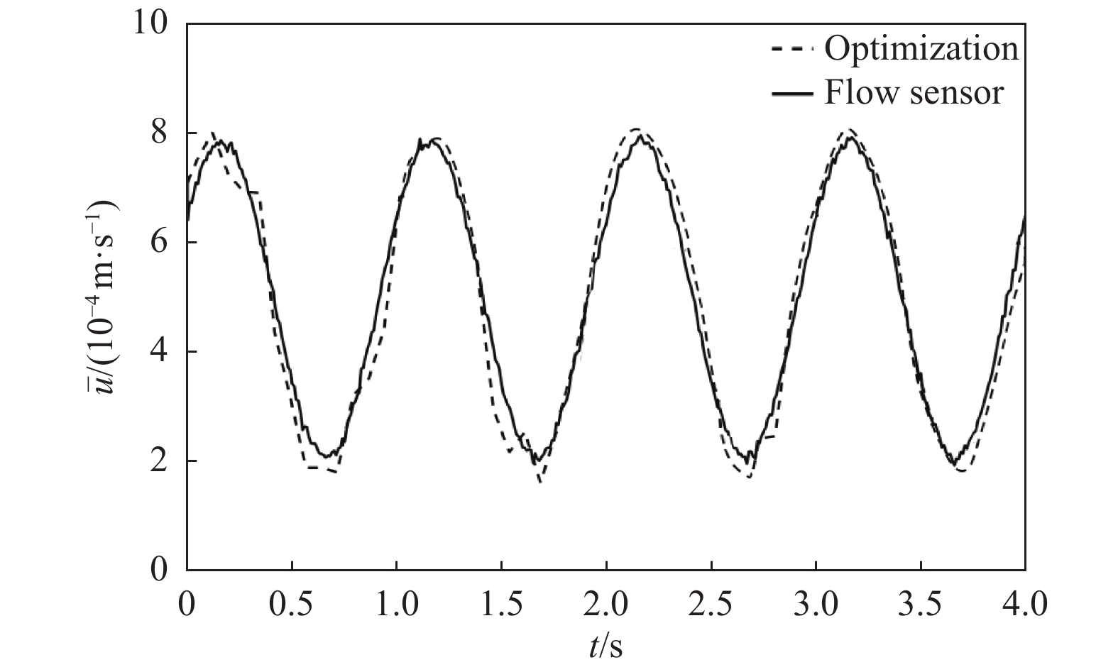
提取实验所得图像序列的灰度值,进行滤波降噪处理并转换为对应浓度值,代入优化算法式子中求解微通道内的平均流速。在相同条件下利用流量传感器测量微通道内的实时流量,用测量结果除以微通道横截面积得到微通道内的流速。将上述两种方法测得的流速结果进行对比,如图9所示。可以看出:优化算法所得流速与使用传感器测量计算的结果基本一致,速度变化的频率预测准确,幅值存在一定误差,相关系数为0.9814。
![]() 图 9 优化算法与流量传感器测量计算结果对比Fig. 9 Comparison of the average velocity derived by the optimization algorithm and the experimental measurement by the flow sensor
图 9 优化算法与流量传感器测量计算结果对比Fig. 9 Comparison of the average velocity derived by the optimization algorithm and the experimental measurement by the flow sensor4 结 论
本文提出了基于时空浓度梯度反演扁平微通道中平均流速的优化算法。无噪声条件下优化算法反演结果几乎无误差;噪声条件下,增大浓度信号的频率与振幅、采用扩散系数较小的物质可以提升算法的准确度;优化算法反演结果与流量传感器测量计算结果进行比较,相关系数为0.9814。本文提出的方法操作简便、精度较高,是一种行之有效的微通道流速测量手段。
-
![]()
图 3 微通道内浓度分布仿真结果
Fig. 3 Simulation results of the concentration distribution in the micro-channel
![]()
图 4 直接反演法和优化算法求得平均流速与真实流速对比
Fig. 4 Comparison between the real velocity and the average velocity derived based on the direct inversion method and the optimiza-tion algorithm
![]()
图 5 浓度信号参数对优化算法反演平均流速的影响
Fig. 5 Influence of parameters of the concentration signals on the average velocity derived by the optimization algorithm
-
[1] WOOTTON R C R,DEMELLO A J. Microfluidics: Exploiting ele-phants in the room[J]. Nature,2010,464(7290):839-840. doi: 10.1038/464839a
[2] LUCCHETTA D E,VITA F,FRANCESCANGELI D,et al. Optical measurement of flow rate in a microfluidic channel[J]. Microfluidics and Nanofluidics,2016,20(1):9-13. doi: 10.1007/s10404-015-1690-1
[3] PATERLINI-BRECHOT P,BENALI N L. Circulating tumor cells (CTC) detection: Clinical impact and future directions[J]. Cancer Letters,2007,253(2):180-204. doi: 10.1016/j.canlet.2006.12.014
[4] LEI X,LIU B,WU H,et al. The effect of fluid shear stress on fibroblasts and stem cells on plane and groove topographies[J]. Cell Adhesion & Migration,2020,14(1):12-23. doi: 10.1080/19336918.2020.1713532
[5] LI Y,QIN Z,ZHOU L,et al. Collective influence of substrate chemistry with physiological fluid shear stress on human umbilical vein endothelial cells[J]. Cell Biology International,2021:1926-1934. doi: 10.1002/cbin.11632
[6] LIU Y O,KLAAS M,SCHRÖDER W. Measurements of the wall-shear stress distribution in turbulent channel flow using the micro-pillar shear stress sensor MPS3[J]. Experimental Thermal and Fluid Science,2019,106:171-182. doi: 10.1016/j.expthermflusci.2019.04.022
[7] KOO H J,VELEV O D. Design and characterization of hydrogel-based microfluidic devices with biomimetic solute transport net-works[J]. Biomicrofluidics,2017,11(2):104-116. doi: 10.1063/1.4978617
[8] SINTON D. Microscale flow visualization[J]. Microfluidics and Nanofluidics,2004,1(1):2-21. doi: 10.1007/s10404-004-0009-4
[9] KOVALEV A V,YAGODNITSYNA A A,BILSKY A V. Micro-PTV technique application to velocity field measurements in immis-cible liquid-liquid plug flow in microchannels[J]. Journal of Physics: Conference Series,2019,1421:012026. doi: 10.1088/1742-6596/1421/1/012026
[10] QURESHI M H,TIEN W H,LIN Y J P. Performance comparison of particle tracking velocimetry (PTV) and particle image velocimetry (PIV) with long-exposure particle streaks[J]. Measurement Science and Technology,2021,32(2):024008. doi: 10.1088/1361-6501/abb747
[11] 黄湛. 标量图像测速原理及数值检验[J]. 实验流体力学,2009,23(2):87-93. DOI: 10.3969/j.issn.1672-9897.2009.02.019 HUANG Z. The theory and DNS testing of scalar image velocime-try[J]. Journal of Experiments in Fluid Mechanics,2009,23(2):87-93. doi: 10.3969/j.issn.1672-9897.2009.02.019
[12] WERELEY S T,MEINHART C D. Recent advances in micro-particle image velocimetry[J]. Annual Review of Fluid Mechanics,2010,42(1):557-576. doi: 10.1146/annurev-fluid-121108-145427
[13] TANG M,LIU F,LEI J,et al. Simple and convenient microfluidic flow rate measurement based on microbubble image velocimetry[J]. Microfluidics and Nanofluidics,2019,23(11):118-126. doi: 10.1007/s10404-019-2285-z
[14] KIM C S,KIM W,LEE K,et al. High-speed color three-dimensional measurement based on parallel confocal detection with a focus tunable lens[J]. Optics Express,2019,27(20):28466-28479. doi: 10.1364/OE.27.028466
[15] GILLISSEN J J,VILQUIN A,KELLAY H,et al. A space–time in-tegral minimisation method for the reconstruction of velocity fields from measured scalar fields[J]. Journal of Fluid Mechanics,2018,854:348-366. doi: 10.1017/jfm.2018.559
[16] SHELBY J P,CHIU D T. Mapping fast flows over micrometer-length scales using flow-tagging velocimetry and single-molecule detec-tion[J]. Analytical Chemistry,2003,75(6):1387-1392. doi: 10.1021/ac026275+
[17] MAYNES D,WEBB A R. Velocity profile characterization in sub-millimeter diameter tubes using molecular tagging velocimetry[J]. Experiments in Fluids,2002,32(1):3-15. doi: 10.1007/s003480200001
[18] 覃开蓉,柳兆荣,徐刚. 具有切应力梯度的平行平板流动腔的构造[J]. 力学季刊,2001,22(3):281-288. DOI: 10.3969/j.issn.0254-0053.2001.03.002 QIN K R,LIU Z R,XU G. Construction of parallel-plate flow Chambers with shear stress gradients[J]. Chinese Quarterly of Mecha-nics,2001,22(3):281-288. doi: 10.3969/j.issn.0254-0053.2001.03.002
[19] LI Y J,LI Y,CAO T,et al. Transport of dynamic biochemical signals in steady flow in a shallow Y-shaped microfluidic channel: effect of transverse diffusion and longitudinal dispersion[J]. Journal of Biome-chanical Engineering,2013,135(12):121011. doi: 10.1115/1.4025774
[20] 徐刚,覃开蓉,柳兆荣. 平行平板流动腔脉动流切应力的计算[J]. 力学季刊,2000,21(1):45-51. DOI: 10.15959/j.cnki.0254-0053.2000.01.009 XU G,QIN K R,LIU Z R. Calculation of the shear stress in the parallel-plate flow chamber under pulsatile flow condition[J]. Chi-nese Quarterly of Mechanics,2000,21(1):45-51. doi: 10.15959/j.cnki.0254-0053.2000.01.009
-
期刊类型引用(0)
其他类型引用(2)
 下载:
下载:


计量
- 文章访问数: 603
- HTML全文浏览量: 242
- PDF下载量: 50
- 被引次数: 2